38 excel chart data labels outside end

Excel Pivot Table DrillDown Show Details Show Records With DrillDown . When you summarize your data by creating an Excel Pivot Table, each number in the Values area represents one or more records in the pivot table source data.In the screen shot below, the selected cell is the total count of new customers for the East region in 2014. Position labels in a paginated report chart - Microsoft ... On the design surface, right-click the chart and select Show Data Labels. Open the Properties pane. On the View tab, click Properties On the design surface, click the series. The properties for the series are displayed in the Properties pane. In the Data section, expand the DataPoint node, then expand the Label node.

Questions from Tableau Training: Can I Move Mark Labels ... Now, Tableau has moved every label to the bottom left of each point on the line chart. This option has overridden the default, therefore mark labels can overlap our line (as seen above). I'll leave it to you to explore the best option for your scenario. Finally, we have the pie chart: one in which labels are often used!

Excel chart data labels outside end

Solved: How can I get data labels to show for each column ... Turn on 'Overflow text' under Data label' Format tab. Also, you can adjust the position of the Data Label by switching to 'Outside End' or 'Inside Center' so that your Data Label gets displayed properly. If this post helps, then mark it as 'Accept as Solution ' so that it could help others. Regards, Sanket Bhagwat View solution in original post How to Create Bar of Pie Chart in Excel Tutorial! Here you can decide the position or alignment of the data labels. For example, if you check 'outside end' on the checklist option, the data label will appear outside the pie chart. Step 10: You can click and drag on the highlighted slice percentage value to position it anywhere on the chart with leader lines to show where it is originating from. 38 excel chart move data labels How to add data labels from different column in an Excel ... Right click the data series in the chart, and select Add Data Labels > Add Data Labels from the context menu to add data labels. 2. Click any data label to select all data labels, and then click the specified data label to select it only in the chart. 3.

Excel chart data labels outside end. Custom Chart Data Labels In Excel With Formulas Follow the steps below to create the custom data labels. Select the chart label you want to change. In the formula-bar hit = (equals), select the cell reference containing your chart label's data. In this case, the first label is in cell E2. Finally, repeat for all your chart laebls. Bar Chart - Microsoft Tech Community I am recreating a column bar chart in Excel that was on a PDF. I need to have the totals just above the colored bars in the chart. ... Labels: Charting; Excel ... On the Chart Design tab of the ribbon, select add chart Element > Data Labels > Outside End. 0 Likes . Reply. Share. Share to LinkedIn; Share to Facebook; Share to Twitter; Share to ... Display data point labels outside a pie chart in a ... On the design surface, right-click on the chart and select Show Data Labels. To display data point labels outside a pie chart Create a pie chart and display the data labels. Open the Properties pane. On the design surface, click on the pie itself to display the Category properties in the Properties pane. Expand the CustomAttributes node. Excel Data Bars Conditional Formatting On the Ribbon, click the Home tab, and then in the Styles group, click Conditional Formatting. In the list of conditional formatting options, click Data Bars, and then click one of the Data Bar options -- Gradient Fill or Solid Fill. (see tips below) The selected cells now show Data Bars, along with the original numbers.

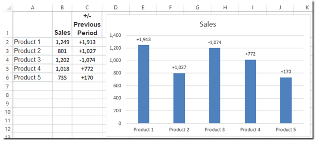
How to color chart bars based on their values Press with mouse on "Select Data...", a dialog box appears. Press with left mouse button on the "Edit" button. Another dialog box shows up on the screen. Select cell range B3:D26. Press Enter, press with left mouse button on "OK" button. You are now back to the first dialog box. Press with left mouse button on "OK" button to dismiss the dialog box. How to change Excel table styles and remove table ... On the Design tab, in the Table Styles group, click the More button. Underneath the table style templates, click Clear. Tip. To remove a table but keep data and formatting, go to the Design tab Tools group, and click Convert to Range. Or, right-click anywhere within the table, and select Table > Convert to Range. How to Make a Bar Graph in Excel (Clustered & Stacked Charts) To see one of these elements in action, click Data Labels > Outside End. Now viewers can see the exact value of each bar. There are tons of options here, from axis labels to trend lines. If you want to add or remove anything from your chart, check here first! Kasper Langmann, Co-founder of Spreadsheeto Structured references in Excel tables - Ablebits Structured references can be used in formulas both inside and outside an Excel table, which makes locating tables in large workbooks easier. Formula auto-fill (calculated columns) To perform the same calculation in each table row, it is enough to enter a formula in just one cell.

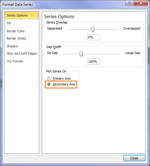
Data Labels bar chart - inside end if negative and outside ... (A stacked column chart has the overlap set to 100% by default, but it doesn't allow outside end data labels.) I added my data labels, and positioned them outside or inside end. If you want the bars to look the same, you can apply the same color to both sets. You must log in or register to reply here. Similar threads J How to make a scatter plot in Excel - Ablebits Select the Value From Cells box, and then select the range from which you want to pull data labels (B2:B6 in our case). If you'd like to display only the names, clear the X Value and/or Y Value box to remove the numeric values from the labels. Specify the labels position, Above data points in our example. That's it! Stacked Waterfall Chart with Positive and Negative Values ... I am trying to create a stacked waterfall chart in Excel that behaves this way when there are positive and negative values: (taken from here: Peltier Tech Split Bar Waterfall Chart - Peltier Tech) In Excel 2019, the closest I have been able to get is the following when using the built-in waterfall chart feature: Pie of Pie Chart in Excel - Inserting, Customizing - Excel ... This is going to open a Format Data Labels pane at the right of excel. Mark the percentage, category name, and legend key. Select the position of data labels at Outside End. Select the fill color for data labels as white as we will change the chart background in the coming section. You can do it from the fill tab of the opened pane.

Axis Labels That Don't Block Plotted Data - Peltier Tech Blog

How to Create A Timeline Graph in Excel [Tutorial & ... Go to Label Options and then change Label Contains to Category Name only. Change the Label Position to Outside End. Now select the horizontal axis on the chart and hit delete on the keyboard. You should now see your actions as labels at the end of the lines touching the horizontal line. The dates will show below the horizontal line.

Format Number Options for Chart Data Labels in Excel 2011 for Mac

Chart.ApplyDataLabels method (Excel) | Microsoft Docs For the Chart and Series objects, True if the series has leader lines. Pass a Boolean value to enable or disable the series name for the data label. Pass a Boolean value to enable or disable the category name for the data label. Pass a Boolean value to enable or disable the value for the data label.

Format data labels in a chart in Office 2016 for Mac - Office Support

Buttons For Inserting Images Or Charts In Excel Greyed Out? Click "For objects, show all" within the Excel options. Within the Excel settings you can choose if objects (including charts and images) should be shown in your workbook. If this setting is set to hide all objects, you cannot insert any new objects so that the buttons are greyed-out. The setting is called "For objects, show:".

Excel Custom Chart Labels • My Online Training Hub

Instructions for NP EX19 4a - Alanis Parks Department ... Modify the chart in the range G2:O20 as follows: a. Enter 2018 Park Spending as Percentage of Total as the chart title. b. Change the data labels to include the Category as well as the Percentage, and position the labels in the Outside End location. c. Remove the Legend from the chart.

How to edit the label of a chart in Excel? - Stack Overflow

Excel Waterfall Chart: How to Create One That Doesn't Suck Ideally, you would create a waterfall chart the same way as any other Excel chart: (1) click inside the data table, (2) click in the ribbon on the chart you want to insert. ... in Excel 2016 Microsoft decided to listen to user feedback and introduced 6 highly requested charts in Excel 2016, including a built-in Excel waterfall chart.

How to Add Data Labels in an Excel Chart in Excel 2010 - YouTube

Controlling Chart Gridlines (Microsoft Excel) Select the chart by clicking on it. You should see selection handles appear around the outside of the chart. Make sure that the Layout tab of the ribbon is displayed. (This tab is only visible when you've selected the chart in step 1.) Click the Gridlines tool in the Axes group. You'll see a drop-down menu appear with various options.

Solution - Challenge 19 – Make Comparative Horizontal Bar Graph | `E for Excel | Excel, VBA ...

Series.DataLabels method (Excel) | Microsoft Docs Return value. Object. Remarks. If the series has the Show Value option turned on for the data labels, the returned collection can contain up to one label for each point. Data labels can be turned on or off for individual points in the series. If the series is on an area chart and has the Show Label option turned on for the data labels, the returned collection contains only a single label ...

charts - Excel, giving data labels to only the top/bottom X% values - Stack Overflow

Excel tutorial: build a dynamic bump chart of the English ... This contains a loop which runs over all of the lines (series) in the active chart and formats them to be thin grey lines with the team names added as a data label: Now that your Excel file contains VBA, you'll need to Save As and select the macro-enabled file .xlsm. Click the chart area and move it in to give the data labels more room. 8.

How to Make Excel Charts More Intuitive by Adding Data Labels and Tables - Data Recovery Blog

DataLabel.Position property (Excel) | Microsoft Docs In this article. Returns or sets an XlDataLabelPosition value that represents the position of the data label.. Syntax. expression.Position. expression A variable that represents a DataLabel object.. Support and feedback. Have questions or feedback about Office VBA or this documentation?

Adobe Using RoboHelp HTML 11 Robo Help 11.0 Operation Manual En

38 excel chart move data labels How to add data labels from different column in an Excel ... Right click the data series in the chart, and select Add Data Labels > Add Data Labels from the context menu to add data labels. 2. Click any data label to select all data labels, and then click the specified data label to select it only in the chart. 3.

Excel Line Charts – Standard, Stacked – Free Template Download - Automate Excel

How to Create Bar of Pie Chart in Excel Tutorial! Here you can decide the position or alignment of the data labels. For example, if you check 'outside end' on the checklist option, the data label will appear outside the pie chart. Step 10: You can click and drag on the highlighted slice percentage value to position it anywhere on the chart with leader lines to show where it is originating from.