41 excel pie chart add labels

Pie Chart in Excel - Inserting, Formatting, Filters, Data Labels To add Data Labels, Click on the + icon on the top right corner of the chart and mark the data label checkbox. You can also unmark the legends as we will add legend keys in the data labels. We can also format these data labels to show both percentage contribution and legend:- Right click on the Data Labels on the chart. spreadsheetplanet.com › bar-of-pie-chart-excelHow to Create Bar of Pie Chart in Excel? Step-by-Step Excel lets us add our own customizations to the Bar of Pie chart. For example, it lets us specify how we want the portions to get split between the pie and the stacked bar. It also lets us specify whether we want to display data labels, what data labels we want to be displayed as well as what formatting and styling we want to apply to the labels.

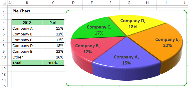
Pie Chart Examples | Types of Pie Charts in Excel with Examples If we add the labels, then it will show what categories cover the sub Pie chart. The pie chart has school fees and savings, representing as other in the main part chart. 3. Bar of PIE Chart ... Here we discuss Types of Pie Chart in Excel along with practical examples and downloadable excel template. You can also go through our other suggested ...

Excel pie chart add labels

How to Create a Pie Chart in Excel | Smartsheet Enter data into Excel with the desired numerical values at the end of the list. Create a Pie of Pie chart. Double-click the primary chart to open the Format Data Series window. Click Options and adjust the value for Second plot contains the last to match the number of categories you want in the "other" category. › ms-excel-pie-chartHow to Make a Pie Chart in Excel (Only Guide You Need) Sep 13, 2021 · To add labels to the slices of the pie chart do the following. 1 st select the pie chart and press on to the “+” shaped button which is actually the Chart Elements option Then put a tick mark on the Data Labels You will see that the data labels are inserted into the slices of your pie chart. Add a DATA LABEL to ONE POINT on a chart in Excel All the data points will be highlighted. Click again on the single point that you want to add a data label to. Right-click and select ' Add data label '. This is the key step! Right-click again on the data point itself (not the label) and select ' Format data label '. You can now configure the label as required — select the content of ...

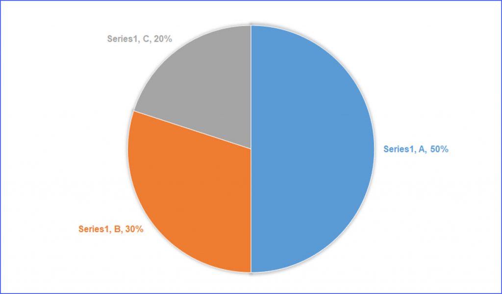
Excel pie chart add labels. Pie of Pie Chart in Excel – Inserting, Customizing, Formatting Jan 03, 2022 · Pie of Pie Chart in Excel contains two pie charts in which one pie chart is a subset of another pie chart. It is subset of Pie chart in excel. ... As we can see, the chart is slightly hard to read as there are no values or percentage ratios on the chart. To add the data labels:-Select the chart and click on + icon at the top right corner of chart. Pie Chart in Excel | How to Create Pie Chart | Step-by-Step Guide to Excel Pie Chart. Here we discuss how to use Pie Chart in Excel along with practical examples and downloadable excel template. EDUCBA. MENU MENU. ... Step 10: Now, right-click on one of the slices of the pie and select add data labels. This will add all the values we are showing on the slices of the pie. Step 11: ... Microsoft Excel Tutorials: Add Data Labels to a Pie Chart You should get the following menu: From the menu, select Add Data Labels. New data labels will then appear on your chart: The values are in percentages in Excel 2007, however. To change this, right click your chart again. From the menu, select Format Data Labels: When you click Format Data Labels , you should get a dialogue box. Inserting Data Label in the Color Legend of a pie chart Small and Medium Business. Public Sector. Internet of Things (IoT) Azure Partner Community. Expand your Azure partner-to-partner network. Microsoft Tech Talks. Bringing IT Pros together through In-Person & Virtual events. MVP Award Program. Find out more about the Microsoft MVP Award Program.

Excel 2010 pie chart data labels in case of "Best Fit" Based on my tested in Excel 2010, the data labels in the "Inside" or "Outside" is based on the data source. If the gap between the data is big, the data labels and leader lines is "outside" the chart. And if the gap between the data is small, the data labels and leader lines is "inside" the chart. Regards, George Zhao. TechNet Community Support. How to make a pie chart in Excel - ablebits.com Nov 12, 2015 · Adding data labels to Excel pie charts. In this pie chart example, we are going to add labels to all data points. To do this, click the Chart Elements button in the upper-right corner of your pie graph, and select the Data Labels option. Additionally, you may want to change the Excel pie chart labels location by clicking the arrow next to Data ... How to Create Bar of Pie Chart in Excel? Step-by-Step How to Customize a Bar of Pie Chart. Excel lets us add our own customizations to the Bar of Pie chart. For example, it lets us specify how we want the portions to get split between the pie and the stacked bar. ... To add and format data labels to portions in your Bar of pie chart, follow the steps below: Click anywhere on the blank area of the ... Multiple data labels (in separate locations on chart) You can do it in a single chart. Create the chart so it has 2 columns of data. At first only the 1 column of data will be displayed. Move that series to the secondary axis. You can now apply different data labels to each series. Attached Files 819208.xlsx‎ (13.8 KB, 263 views) Download Cheers Andy Register To Reply

Adding data labels to a pie chart - OzGrid Free Excel/VBA Help Forum Re: Adding data labels to a pie chart. Thanks again, norie. Really appreciate the help. I tried recording a macro while doing it manually (before my first post). But it didn't record anything about labels, much less making them bold. › 2015/11/12 › make-pie-chart-excelHow to make a pie chart in Excel - ablebits.com Nov 12, 2015 · Adding data labels to Excel pie charts. In this pie chart example, we are going to add labels to all data points. To do this, click the Chart Elements button in the upper-right corner of your pie graph, and select the Data Labels option. Additionally, you may want to change the Excel pie chart labels location by clicking the arrow next to Data ... Add data labels and callouts to charts in Excel 365 | EasyTweaks.com The steps that I will share in this guide apply to Excel 2021 / 2019 / 2016. Step #1: After generating the chart in Excel, right-click anywhere within the chart and select Add labels . Note that you can also select the very handy option of Adding data Callouts. › pie-chart-examplesPie Chart Examples | Types of Pie Charts in Excel ... - EDUCBA It is similar to Pie of the pie chart, but the only difference is that instead of a sub pie chart, a sub bar chart will be created. With this, we have completed all the 2D charts, and now we will create a 3D Pie chart. 4. 3D PIE Chart. A 3D pie chart is similar to PIE, but it has depth in addition to length and breadth.

How to Add Data Labels to an Excel 2010 Chart - dummies

support.microsoft.com › en-us › officeAdd a pie chart - support.microsoft.com To switch to one of these pie charts, click the chart, and then on the Chart Tools Design tab, click Change Chart Type. When the Change Chart Type gallery opens, pick the one you want. See Also. Select data for a chart in Excel. Create a chart in Excel. Add a chart to your document in Word. Add a chart to your PowerPoint presentation

Excel 3-D Pie Charts - Microsoft Excel 2013

Edit titles or data labels in a chart - support.microsoft.com On a chart, click the label that you want to link to a corresponding worksheet cell. On the worksheet, click in the formula bar, and then type an equal sign (=). Select the worksheet cell that contains the data or text that you want to display in your chart. You can also type the reference to the worksheet cell in the formula bar.

How to Make Labels the Same Color as the Pies in Pie Chart - ExcelNotes

How to Make a Pie Chart in Excel (Only Guide You Need) Sep 13, 2021 · To add labels to the slices of the pie chart do the following. 1 st select the pie chart and press on to the “+” shaped button which is actually the Chart Elements option Then put a tick mark on the Data Labels You will see that the data labels are inserted into the …

Microsoft Excel Tutorials: Add Data Labels to a Pie Chart

c# - Add data labels to excel pie chart - Stack Overflow I am drawing a pie chart with some data: private void DrawFractionChart(Excel.Worksheet activeSheet, Excel.ChartObjects xlCharts, Excel.Range xRange, Excel.Range yRange) { Excel.ChartObject ... Adding labels to markers in Excel from a column in C#. Related. 957.NET String.Format() to add commas in thousands place for a number.

Excel 3-D Pie Charts

How To Make A Pie Chart In Excel: In Just 2 Minutes [2022] When you first create a pie chart, Excel will use the default colors and design.. But if you want to customize your chart to your own liking, you have plenty of options. The easiest way to get an entirely new look is with chart styles.. In the Design portion of the Ribbon, you’ll see a number of different styles displayed in a row. Mouse over them to see a preview:

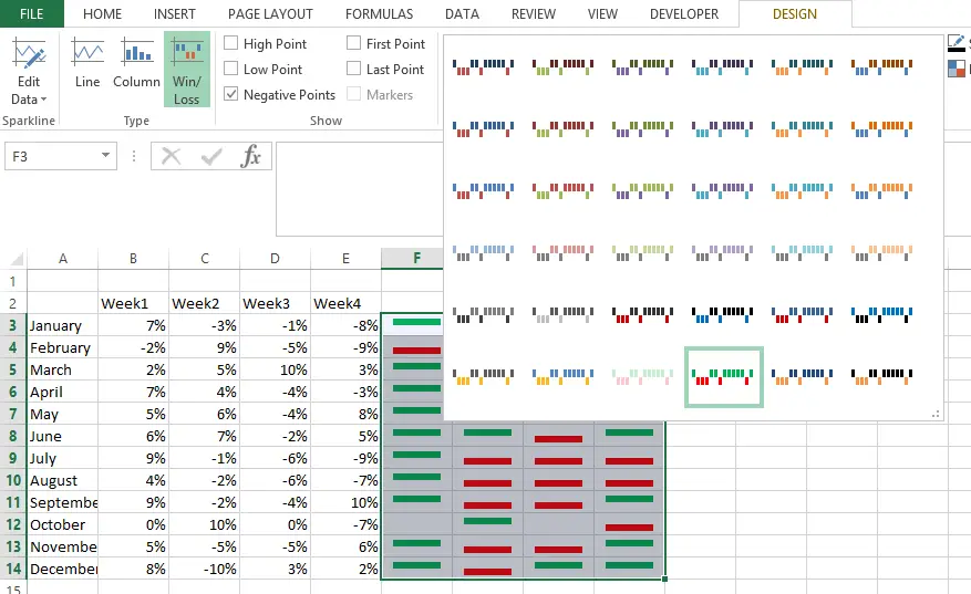
Win Loss Chart in Excel - DataScience Made Simple

How to display leader lines in pie chart in Excel? - ExtendOffice To display leader lines in pie chart, you just need to check an option then drag the labels out. 1. Click at the chart, and right click to select Format Data Labels from context menu. 2. In the popping Format Data Labels dialog/pane, check Show Leader Lines in the Label Options section. See screenshot: 3. Close the dialog, now you can see some ...

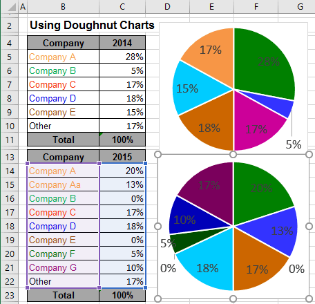
Using Pie Charts and Doughnut Charts in Excel

Excel charts: add title, customize chart axis, legend and data labels ... Click the Chart Elements button, and select the Data Labels option. For example, this is how we can add labels to one of the data series in our Excel chart: For specific chart types, such as pie chart, you can also choose the labels location. For this, click the arrow next to Data Labels, and choose the option you want.

Share :