40 excel pivot table column labels

How to Flatten Data in Excel Pivot Table? - GeeksforGeeks Select a range that you want to flatten - typically, a column of labels. Highlight the empty cells only - hit F5 (GoTo) and select Special > Blanks. Type equals (=) and then the Up Arrow to enter a formula with a direct cell reference to the first data label. Instead of hitting enter, hold down Control and hit Enter. Excel 2016 Pivot table Row and Column Labels - Microsoft Community In Excel 2016 I've found when I create a pivot table it unhelpfully shows 'Row Labels' and 'Column Labels' instead of my field names, although in the top left cell it says 'Count of' and then inserts the correct field name. Years ago when I last used Excel it automatically put the field names in all three heading cells.

Pivot table row labels side by side - Excel Tutorials - OfficeTuts Excel You can copy the following table and paste it into your worksheet as Match Destination Formatting. Now, let's create a pivot table ( Insert >> Tables >> Pivot Table) and check all the values in Pivot Table Fields. Fields should look like this. Right-click inside a pivot table and choose PivotTable Options…. Check data as shown on the image below.

Excel pivot table column labels

Excel filtering pivot table filter/slicer across column label Excel filtering pivot table filter/slicer across column label. Hello. I have a table with the year as the column headings/labels (2009-2021) and a couple other columns with additional information that aren't a year. The rows represent the specific data for each year. I have made a pivot table and slicers for the columns with the other date but ... How to make row labels on same line in pivot table? - ExtendOffice Make row labels on same line with PivotTable Options You can also go to the PivotTable Options dialog box to set an option to finish this operation. 1. Click any one cell in the pivot table, and right click to choose PivotTable Options, see screenshot: 2. Hide Pivot Table Buttons and Labels - Contextures Blog Right-click a cell in the pivot table and, in the pop up menu, click PivotTable Options. In the Display section, remove the check mark from Show Expand/Collapse Buttons. This change will hide the Expand/Collapse buttons to the left of the outer Row Labels and Column Labels. Next, remove the check mark from Display Field Captions and Filter Drop ...

Excel pivot table column labels. How to rename group or row labels in Excel PivotTable? - ExtendOffice To rename Row Labels, you need to go to the Active Field textbox. 1. Click at the PivotTable, then click Analyze tab and go to the Active Field textbox. 2. Now in the Active Field textbox, the active field name is displayed, you can change it in the textbox. Centre Column Headings in Excel Pivot Table To centre the column headings in Excel 2007: Select a cell in the pivot table. On the Ribbon, under the PivotTable Tools tab, click Options. At the far left, in the PivotTable group, click Options. On the Layout & Format tab, in the Layout section, add a check mark to Merge and Center Cells With Labels. Click OK. excel - Custom column labels in PivotTable - Stack Overflow Select the data from which the pivot table is from highlight the column in which the "b" is in find and replace all the "b" with "In Progress" Update the Pivot table OR Copy the data from the pivot table and Paste it as text delimited I believe. -Change the "b" to "In Progress" Please respond if it isnt clear so I can go into further detail. Data Labels in Excel Pivot Chart (Detailed Analysis) 7 Suitable Examples with Data Labels in Excel Pivot Chart Considering All Factors 1. Adding Data Labels in Pivot Chart 2. Set Cell Values as Data Labels 3. Showing Percentages as Data Labels 4. Changing Appearance of Pivot Chart Labels 5. Changing Background of Data Labels 6. Dynamic Pivot Chart Data Labels with Slicers 7.

How To Remove Column Labels In Pivot Table | Brokeasshome.com How to delete a pivot table in excel easy step by guide how to remove pivot table but keep data step by guide delete a pivottable hide pivot table ons and labels contextures blog Share this: Click to share on Twitter (Opens in new window) How to Use Excel Pivot Table Label Filters - Contextures Excel Tips You can use a similar technique to hide most of the items in the Row Labels or Column Labels. Select the pivot table items that you want to keep visible Right-click on one of the selected items In the pop-up menu, click Filter, then click Keep Only Selected Items. All but the selected items are immediately hidden in the pivot table. Excel tutorial: How to rename fields in a pivot table Either right-click on the field and choose Value field settings, or click Field Settings on the Options Tab of the PivotTable Tools ribbon. Here, you can see the original field name. In contrast to value fields, Row and Column label field names will be identical to the name in the field list. In fact, they are linked, as we'll see in a minute. How to make row labels on same line in pivot table? - ExtendOffice Make row labels on same line with PivotTable Options You can also go to the PivotTable Options dialog box to set an option to finish this operation. 1. Click any one cell in the pivot table, and right click to choose PivotTable Options, see screenshot: 2.

Repeat item labels in a PivotTable - support.microsoft.com Right-click the row or column label you want to repeat, and click Field Settings. Click the Layout & Print tab, and check the Repeat item labels box. Make sure Show item labels in tabular form is selected. Notes: When you edit any of the repeated labels, the changes you make are applied to all other cells with the same label. Shifting Row Sub label to another column in Pivot Table Top X in Excel/PowerPivot Pivot Table Filtered by Column Label. 1. Excel Pivot Sub total columns. 0. Pivot table custom sub total. 4. ... How to put Sums in Row Labels. 0. Repeat first layer column headers in Excel Pivot Table. 2. Convert two column list to a table in excel. Hot Network Questions Travelling with a super off-peak train ticket How To Filter Column Labels With VBA In An Excel Pivot Table 1. In Excel I have been able to filter the row labels in a pivot table with this code: Dim PT as PivotTable Set PT = ActiveSheet.PivotTables ("Pivot1") With PT .ManualUpdate=True .ClearAllFiters .PivotFields ("App").PivotFilters.Add Type:=xlCaptionDoesNotContain, Value1:=" (Blank)" End With. I need to do the same filter for the column labels ... How to Customize Your Excel Pivot Chart Data Labels - dummies The Data Labels command on the Design tab's Add Chart Element menu in Excel allows you to label data markers with values from your pivot table. When you click the command button, Excel displays a menu with commands corresponding to locations for the data labels: None, Center, Left, Right, Above, and Below.

Excel Help: Simple method to make Pivot table

Repeat All Item Labels In An Excel Pivot Table | MyExcelOnline STEP 1: Click in the Pivot Table and choose PivotTable Tools > Options (Excel 2010) or Design (Excel 2013 & 2016) > Report Layouts > Show in Outline/Tabular Form. STEP 2: Now to fill in the empty cells in the Row Labels you need to select PivotTable Tools > Options (Excel 2010) or Design (Excel 2013 & 2016) > Report Layouts > Repeat All Item ...

MVP #10: Making a Pivot table that has labels spread across several columns | Productivity Tips ...

How to Group Columns in Excel Pivot Table (2 Methods) We can create a Pivot Table using the Power Query Editor in excel and thus group columns. Let's have a look at the steps involved in this process. Steps: First, go to the source dataset and press Ctrl + T. Next the Create Table dialog box will pop up. Check the range of the table is specified correctly, then press OK.

How to Insert an Excel Pivot Table - YouTube

Pivot Table column label from horizontal to vertical Pivot Table column label from horizontal to vertical After pivot table and with grouping, some column labels have been showed but the caption is on the top. What i want is put the column header at the left of the row as vertical red text show as below. However, i cannot do this, it said "We cant change this part of pivot table".

Design your Pivot Table in Excel | Excel in Excel

How to reset a custom pivot table row label 3. Insert a column and make it equal to the Problem column. 4. Now go back to your Pivot and refresh it to find the Problem column and the duplicate column you just made. 5. Enter both fields into the pivot table and you will see the duplicate column has the original values while the Problem column maintains the problem labels.

Excel Pivot Table Report - Sort Data in Row & Column Labels & in Values Area, use Custom Lists

Design the layout and format of a PivotTable Change a PivotTable to compact, outline, or tabular form Change the way item labels are displayed in a layout form Change the field arrangement in a PivotTable Add fields to a PivotTable Copy fields in a PivotTable Rearrange fields in a PivotTable Remove fields from a PivotTable Change the layout of columns, rows, and subtotals

How-to Make an Excel Stacked Column Pivot Chart with a Secondary Axis - Excel Dashboard Templates

Automatic Row And Column Pivot Table Labels - How To Excel At Excel Next select Pivot Table option Select a table or range option Select to put your Table on a New Worksheet or on the current one, for this tutorial select the first option Click Ok The Options and Design Tab will appear under the Pivot Table Tool Select the check boxes next to the fields you want to use to add them to the Pivot Table

Create a Pivot Table in Excel - The Complete Beginners Guide - QuickExcel

How to add column labels in pivot table [SOLVED] Add a helper column showing Month Text Just as I have done in Column H 2. Now insert a Pivot Table 3. Put Fields in there required sections in the Pivot table Field List Window just as I have done . 4. Now Select the Row Lable column and Uncheck the Subtotal for Material field option. That's it. Check the attached file:- Attached Files

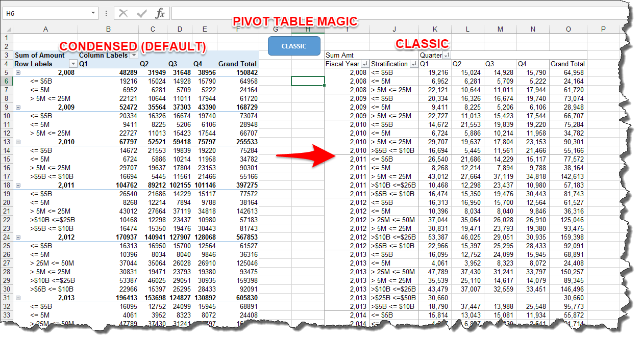
Microsoft Excel — Pivot Table Magic - Let’s Excel - Medium

How to repeat row labels for group in pivot table? - ExtendOffice 1. Firstly, you need to expand the row labels as outline form as above steps shows, and click one row label which you want to repeat in your pivot table. 2. Then right click and choose Field Settings from the context menu, see screenshot: 3. In the Field Settings dialog box, click Layout & Print tab, then check Repeat item labels, see ...

Share :