44 excel graph horizontal axis labels
Use text as horizontal labels in Excel scatter plot Edit each data label individually, type a = character and click the cell that has the corresponding text. This process can be automated with the free XY Chart Labeler add-in. Excel 2013 and newer has the option to include "Value from cells" in the data label dialog. Format the data labels to your preferences and hide the original x axis labels. Scatter chart horizontal axis labels | MrExcel Message Board Apr 26, 2011. #3. Use a Line chart (rather than a XY Scatter chart) and you can have any text in the X values. If you must use a XY Chart, you will have to simulate the effect. Add a dummy series which will have all y values as zero. Then, add data labels for this new series with the desired labels. Locate the data labels below the data points ...
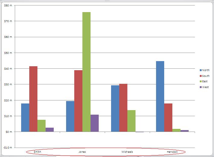
Move Horizontal Axis to Bottom - Excel & Google Sheets Moving X Axis to the Bottom of the Graph. Click on the X Axis; Select Format Axis . 3. Under Format Axis, Select Labels. 4. In the box next to Label Position, switch it to Low. Final Graph in Excel. Now your X Axis Labels are showing at the bottom of the graph instead of in the middle, making it easier to see the labels. Move Horizontal Axis to Bottom in Google Sheets
Excel graph horizontal axis labels
How to Switch (Flip) X & Y Axis in Excel & Google Sheets Switching X and Y Axis. Right Click on Graph > Select Data Range . 2. Click on Values under X-Axis and change. In this case, we’re switching the X-Axis “Clicks” to “Sales”. Do the same for the Y Axis where it says “Series” Change Axis Titles. Similar to Excel, double-click the axis title to change the titles of the updated axes. Text Labels on a Horizontal Bar Chart in Excel - Peltier Tech On the Excel 2007 Chart Tools > Layout tab, click Axes, then Secondary Horizontal Axis, then Show Left to Right Axis. Now the chart has four axes. We want the Rating labels at the bottom of the chart, and we'll place the numerical axis at the top before we hide it. In turn, select the left and right vertical axes. How to rotate axis labels in chart in Excel? - ExtendOffice 1. Right click at the axis you want to rotate its labels, select Format Axis from the context menu. See screenshot: 2. In the Format Axis dialog, click Alignment tab and go to the Text Layout section to select the direction you need from the list box of Text direction. See screenshot: 3. Close the dialog, then you can see the axis labels are rotated. Rotate axis labels in chart of Excel 2013
Excel graph horizontal axis labels. How to Insert Axis Labels In An Excel Chart | Excelchat How to add horizontal axis labels in Excel 2016/2013 We have a sample chart as shown below Figure 2 - Adding Excel axis labels Next, we will click on the chart to turn on the Chart Design tab We will go to Chart Design and select Add Chart Element Figure 3 - How to label axes in Excel How to add axis label to chart in Excel? - ExtendOffice Add axis label to chart in Excel 2013. In Excel 2013, you should do as this: 1. Click to select the chart that you want to insert axis label. 2. Then click the Charts Elements button located the upper-right corner of the chart. In the expanded menu, check Axis Titles option, see screenshot: 3. And both the horizontal and vertical axis text boxes have been added to the chart, then click each of the axis text boxes and enter your own axis labels for X axis and Y axis separately. How to Make Charts and Graphs in Excel | Smartsheet Jan 22, 2018 · In this example, clicking Primary Horizontal will remove the year labels on the horizontal axis of your chart. Click More Axis Options … from the Axes dropdown menu to open a window with additional formatting and text options such as adding tick marks, labels, or numbers, or to change text color and size. Change axis labels in a chart - support.microsoft.com Right-click the category labels you want to change, and click Select Data. In the Horizontal (Category) Axis Labels box, click Edit. In the Axis label range box, enter the labels you want to use, separated by commas. For example, type Quarter 1,Quarter 2,Quarter 3,Quarter 4. Change the format of text and numbers in labels
Change the scale of the horizontal (category) axis in a chart The horizontal (category) axis, also known as the x axis, of a chart displays text labels instead of numeric intervals and provides fewer scaling options than are available for a vertical (value) axis, also known as the y axis, of the chart. However, you can specify the following axis options: Interval between tick marks and labels How to add a line in Excel graph (average line, benchmark ... Sep 12, 2018 · Here is a quick solution: double-click the on the horizontal axis to open the Format Axis pane, switch to Axis Options and choose to position the axis On tick marks: However, this simple method has one drawback - it makes the leftmost and rightmost bars half as thin as the other bars, which does not look nice. Excel tutorial: How to customize axis labels Instead you'll need to open up the Select Data window. Here you'll see the horizontal axis labels listed on the right. Click the edit button to access the label range. It's not obvious, but you can type arbitrary labels separated with commas in this field. So I can just enter A through F. When I click OK, the chart is updated. Add or remove a secondary axis in a chart in Excel A secondary axis can also be used as part of a combination chart when you have mixed types of data (for example, price and volume) in the same chart. In this chart, the primary vertical axis on the left is used for sales volumes, whereas the secondary vertical axis on the right side is for price figures. Do any of the following: Add a secondary ...
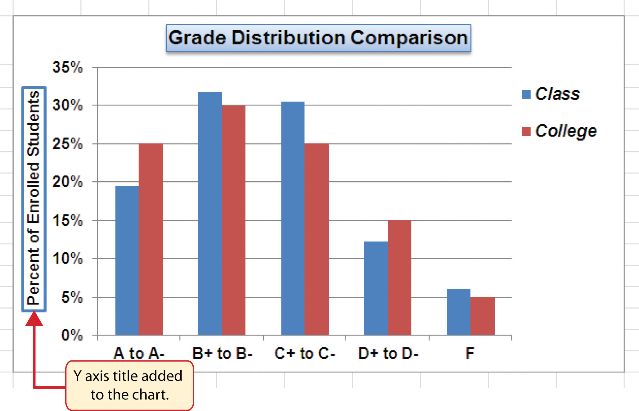
Excel Chart not showing SOME X-axis labels - Super User Apr 05, 2017 · On the sidebar, click on "CHART OPTIONS" and select "Horizontal (Category) Axis" from the drop down menu. Four icons will appear below the menu bar. The right most icon looks like a bar graph. Click that. A navigation bar with several twistys will appear below the icon ribbon. Click on the "LABELS" twisty. How to wrap X axis labels in a chart in Excel? - ExtendOffice We can wrap the labels in the label cells, and then the labels in the chart axis will wrap automatically. And you can do as follows: 1. Double click a label cell, and put the cursor at the place where you will break the label. 2. Add a hard return or carriages with pressing the Alt + Enter keys simultaneously. 3. How-to Highlight Specific Horizontal Axis Labels in Excel Line Charts ... In this video, you will learn how to highlight categories in your horizontal axis for an Excel chart. This is in answer to "I am trying to bold 5 months (ou... How to Add Axis Labels in Excel Charts - Step-by-Step (2022) - Spreadsheeto How to add axis titles 1. Left-click the Excel chart. 2. Click the plus button in the upper right corner of the chart. 3. Click Axis Titles to put a checkmark in the axis title checkbox. This will display axis titles. 4. Click the added axis title text box to write your axis label.
Excel - Line Chart
Axis Labels overlapping Excel charts and graphs - AuditExcel Stop Labels overlapping chart. There is a really quick fix for this. As shown below: Right click on the Axis. Choose the Format Axis option. Open the Labels dropdown. For label position change it to 'Low'. The end result is you eliminate the labels overlapping the chart and it is easier to understand what you are seeing .
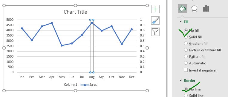
How to remove data labels from Graph? | CanvasJS Charts
Excel Graph - horizontal axis labels not showing properly Open your Excel file. Right-click on the sheet tab. Choose "View Code". Press CTRL-M. Select the downloaded file and import. Close the VBA editor. Select the cells with the confidential data. Press Alt-F8. Choose the macro Anonymize.
30 Label X And Y Axis In Excel - Best Labeling Ideas
How to Make a Bar Graph in Excel: 9 Steps (with Pictures) May 02, 2022 · Add labels for the graph's X- and Y-axes. To do so, click the A1 cell (X-axis) and type in a label, then do the same for the B1 cell (Y-axis). For example, a graph measuring the temperature over a week's worth of days might have "Days" in A1 and "Temperature" in B1.
30 Excel Graph Label Axis - Label Design Ideas 2020
Change axis labels in a chart in Office - support.microsoft.com In charts, axis labels are shown below the horizontal (also known as category) axis, next to the vertical (also known as value) axis, and, in a 3-D chart, next to the depth axis. The chart uses text from your source data for axis labels. To change the label, you can change the text in the source data.

Bar Chart | PatternFly
How to group (two-level) axis labels in a chart in Excel? The Pivot Chart tool is so powerful that it can help you to create a chart with one kind of labels grouped by another kind of labels in a two-lever axis easily in Excel. You can do as follows: 1. Create a Pivot Chart with selecting the source data, and: (1) In Excel 2007 and 2010, clicking the PivotTable > PivotChart in the Tables group on the Insert Tab;
Five tips for enhancing Excel charts - TechRepublic
How to rotate axis labels in chart in Excel? - ExtendOffice 1. Right click at the axis you want to rotate its labels, select Format Axis from the context menu. See screenshot: 2. In the Format Axis dialog, click Alignment tab and go to the Text Layout section to select the direction you need from the list box of Text direction. See screenshot: 3. Close the dialog, then you can see the axis labels are rotated. Rotate axis labels in chart of Excel 2013
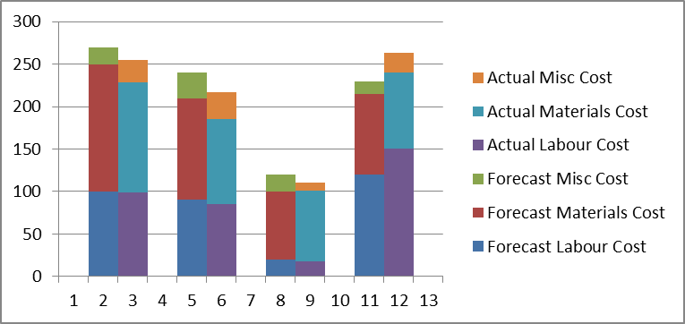
Step-by-step tutorial on creating clustered stacked column bar charts (for free) | Excel Help HQ
Text Labels on a Horizontal Bar Chart in Excel - Peltier Tech On the Excel 2007 Chart Tools > Layout tab, click Axes, then Secondary Horizontal Axis, then Show Left to Right Axis. Now the chart has four axes. We want the Rating labels at the bottom of the chart, and we'll place the numerical axis at the top before we hide it. In turn, select the left and right vertical axes.
Formatting Charts
How to Switch (Flip) X & Y Axis in Excel & Google Sheets Switching X and Y Axis. Right Click on Graph > Select Data Range . 2. Click on Values under X-Axis and change. In this case, we’re switching the X-Axis “Clicks” to “Sales”. Do the same for the Y Axis where it says “Series” Change Axis Titles. Similar to Excel, double-click the axis title to change the titles of the updated axes.

Add horizontal axis labels - VBA Excel - Stack Overflow

Excel: Horizontal Axis Labels as Text - Stack Overflow
34 How To Label Axis In Excel - Labels For You
Resize the Plot Area in Excel Chart - Titles and Labels Overlap - YouTube
35 How To Label The Axis In Excel - Label Design Ideas 2020
Moving X-axis labels at the bottom of the chart below negative values in Excel - PakAccountants.com
How to Insert A Vertical Marker Line in Excel Line Chart
Advanced Chart in Excel - column width based on cell value - Super User

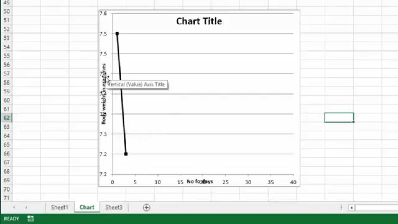
Charting in Excel - Adding Axis Labels - YouTube
Post a Comment for "44 excel graph horizontal axis labels"