43 how to insert data labels in excel pie chart

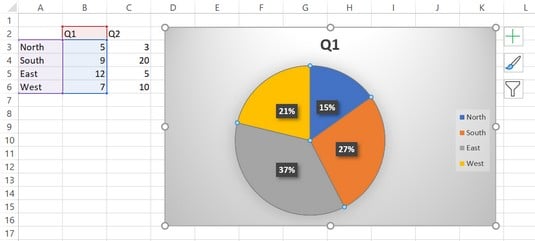
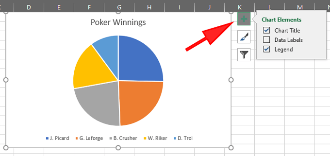
Chart.ApplyDataLabels method (Excel) | Microsoft Learn ApplyDataLabels ( Type, LegendKey, AutoText, HasLeaderLines, ShowSeriesName, ShowCategoryName, ShowValue, ShowPercentage, ShowBubbleSize, Separator) expression A variable that represents a Chart object. Parameters Example This example applies category labels to series one on Chart1. VB Charts ("Chart1").SeriesCollection (1). Create a Pie Chart in Excel (Easy Tutorial) Create the pie chart (repeat steps 2-3). 7. Click the legend at the bottom and press Delete. 8. Select the pie chart. 9. Click the + button on the right side of the chart and click the check box next to Data Labels. 10. Click the paintbrush icon on the right side of the chart and change the color scheme of the pie chart.

Create A Pie Chart In Excel With and Easy Step-By-Step Guide Once you have all your data in place, follow these steps to create a pie chart: Step 1: Select the whole dataset. Step 2: Click on the Insert tab. Step 3: Now, in the charts group, you need to click on the "Insert Pie or Doughnut Chart" option. Step 4: Click on the pie icon that is within the 2-D pie icons.

How to insert data labels in excel pie chart

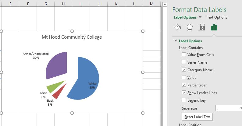
Change the format of data labels in a chart To get there, after adding your data labels, select the data label to format, and then click Chart Elements > Data Labels > More Options. To go to the appropriate area, click one of the four icons ( Fill & Line, Effects, Size & Properties ( Layout & Properties in Outlook or Word), or Label Options) shown here. How to Create a Pie Chart in Excel: A Quick & Easy Guide - wikiHow You need to prepare your chart data in Excel before creating a chart. To make a pie chart, select your data. Click Insert and click the Pie chart icon. Select 2-D or 3-D Pie Chart. Customize your pie chart's colors by using the Chart Elements tab. Click the chart to customize displayed data. Part 1. Creating Pie Chart and Adding/Formatting Data Labels (Excel) Creating Pie Chart and Adding/Formatting Data Labels (Excel) Creating Pie Chart and Adding/Formatting Data Labels (Excel)

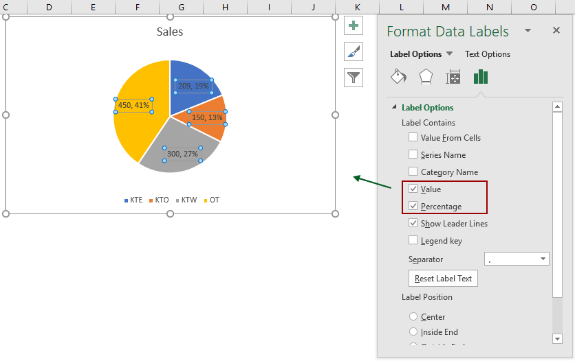
How to insert data labels in excel pie chart. Best Types of Charts in Excel for Data Analysis, Presentation ... Apr 29, 2022 · When your data is represented in ‘percentage’ or ‘part of’, then a pie chart best meets your needs. #4 Use a pie chart to show data composition only when the pie slices are of comparable sizes. In other words, do not use a pie chart if the size of one pie slice completely dwarfs the size of the other pie slice(s): Add data labels and callouts to charts in Excel 365 - EasyTweaks.com The steps that I will share in this guide apply to Excel 2021 / 2019 / 2016. Step #1: After generating the chart in Excel, right-click anywhere within the chart and select Add labels . Note that you can also select the very handy option of Adding data Callouts. Pie Chart in Excel - Inserting, Formatting, Filters, Data Labels To add Data Labels, Click on the + icon on the top right corner of the chart and mark the data label checkbox. You can also unmark the legends as we will add legend keys in the data labels. We can also format these data labels to show both percentage contribution and legend:- Right click on the Data Labels on the chart. Pie Chart in Excel | How to Create Pie Chart - EDUCBA Step 1: Do not select the data; rather, place a cursor outside the data and insert one PIE CHART. Go to the Insert tab and click on a PIE. Step 2: once you click on a 2-D Pie chart, it will insert the blank chart as shown in the below image. Step 3: Right-click on the chart and choose Select Data. Step 4: once you click on Select Data, it will ...

How to Create a SPEEDOMETER Chart [Gauge] in Excel Now, the next thing is to create a pie chart with a third data table to add the needle. For this, right-click on the chart and then click on “Select data”. In the “Select Data Source” window click on “Add” to enter a new “Legend Entries” and select the “Values” column from the third data table. Possible to add second data label to pie chart? - excelforum.com Re: Possible to add second data label to pie chart? You get one data label per plotted point. I think you could use the. first trick in this page of Andy Pope's, and make the pie in front the. same size as the one in back, and use one pie for the outside labels and. the other for the inside labels. How to Make a PIE Chart in Excel (Easy Step-by-Step Guide) Creating a Pie Chart in Excel. To create a Pie chart in Excel, you need to have your data structured as shown below. The description of the pie slices should be in the left column and the data for each slice should be in the right column. Once you have the data in place, below are the steps to create a Pie chart in Excel: Select the entire dataset How to Create a Pie Chart in Excel | Smartsheet Aug 27, 2018 · To create a pie chart in Excel 2016, add your data set to a worksheet and highlight it. Then click the Insert tab, and click the dropdown menu next to the image of a pie chart. Select the chart type you want to use and the chosen chart will appear on the worksheet with the data you selected.

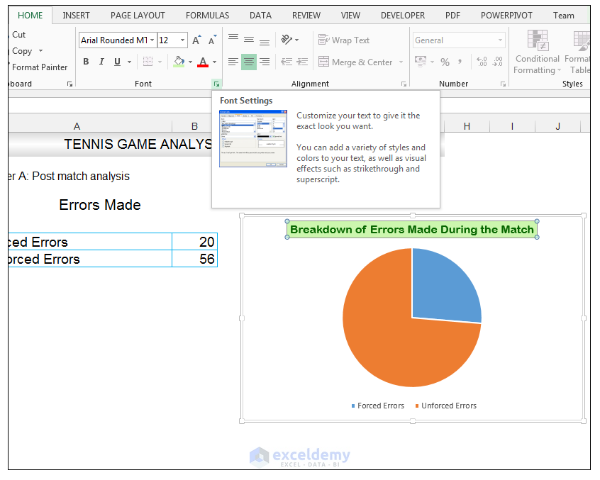
How to Make a Pie Chart in Excel & Add Rich Data Labels to ... Formatting the Data Labels of the Pie Chart 1) In cell A11, type the following text, Main reason for unforced errors, and give the cell a light blue fill and a black border. 2) In cell A12, type the text Sinusitis, and give the cell a black border, and align the text to the center position. Adding data labels to a pie chart - Excel General - OzGrid Free Excel ... Re: Adding data labels to a pie chart. Thanks again, norie. Really appreciate the help. I tried recording a macro while doing it manually (before my first post). But it didn't record anything about labels, much less making them bold. Excel Pie Chart - How to Create & Customize? (Top 5 Types) Step 1: Click on the Pie Chart > click the ' + ' icon > check/tick the " Data Labels " checkbox in the " Chart Element " box > select the " Data Labels " right arrow > select the " More Options… ", as shown below. The " Format Data Labels" pane opens. How to Make a Pie Chart with Multiple Data in Excel (2 Ways) - ExcelDemy First, to add Data Labels, click on the Plus sign as marked in the following picture. After that, check the box of Data Labels. At this stage, you will be able to see that all of your data has labels now. Next, right-click on any of the labels and select Format Data Labels. After that, a new dialogue box named Format Data Labels will pop up.

Automatically Group Smaller Slices in Pie Charts to one big Slice

How to add data labels in excel to graph or chart (Step-by-Step) Add data labels to a chart 1. Select a data series or a graph. After picking the series, click the data point you want to label. 2. Click Add Chart Element Chart Elements button > Data Labels in the upper right corner, close to the chart. 3. Click the arrow and select an option to modify the location. 4.

Add or remove data labels in a chart

Inserting Data Label in the Color Legend of a pie chart Inserting Data Label in the Color Legend of a pie chart. Hi, I am trying to insert data labels (percentages) as part of the side colored legend, rather than on the pie chart itself, as displayed on the image below. Does Excel offer that option and if so, how can i go about it?

Creating Graphs in Excel 2013

excel - Pie Chart VBA DataLabel Formatting - Stack Overflow sub updatechartformat () with activesheet.chartobjects ("chart 4") .activate with .chart.seriescollection (1).datalabels .showpercentage = true .separator = "" & chr (10) & "" end with end with with activesheet.chartobjects ("chart 1") .activate with .chart.seriescollection (1).datalabels .showpercentage = true .showvalue = false …

How to Create and Format a Pie Chart in Excel

How to insert data labels to a Pie chart in Excel 2013 - YouTube How-To Guide 98.4K subscribers This video will show you the simple steps to insert Data Labels in a pie chart in Microsoft® Excel 2013. Content in this video is provided on an "as is"...

5 New Charts to Visually Display Data in Excel 2019 - dummies

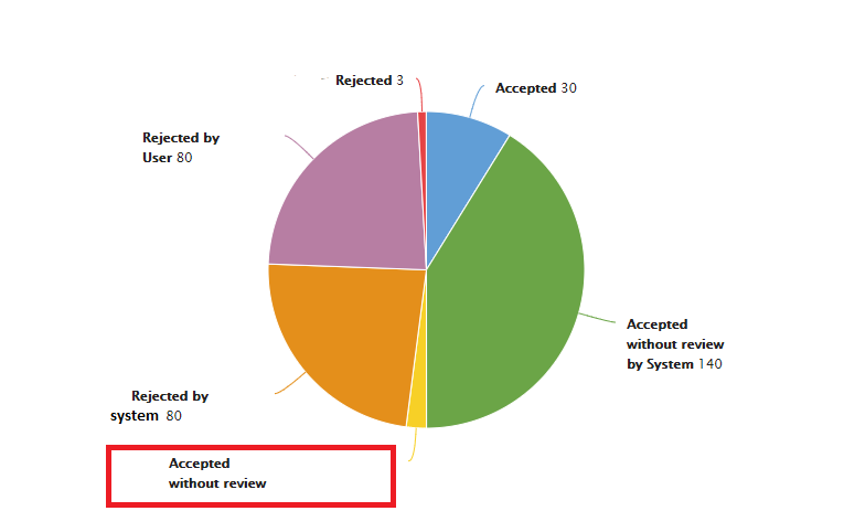
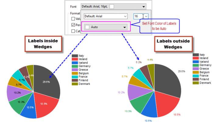
How to Make Pie Chart with Labels both Inside and Outside 1. Right click on the pie chart, click " Add Data Labels "; 2. Right click on the data label, click " Format Data Labels " in the dialog box; 3. In the " Format Data Labels " window, select " value ", " Show Leader Lines ", and then " Inside End " in the Label Position section; Step 10: Set second chart as Secondary Axis: 1.

Pie Chart – Excel Tutorial

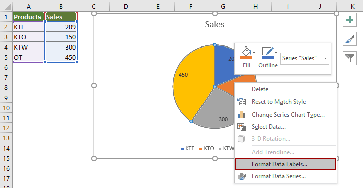
Microsoft Excel Tutorials: Add Data Labels to a Pie Chart - Home and Learn To add the numbers from our E column (the viewing figures), left click on the pie chart itself to select it: The chart is selected when you can see all those blue circles surrounding it. Now right click the chart. You should get the following menu: From the menu, select Add Data Labels. New data labels will then appear on your chart:

Custom data labels in a chart

Add or remove data labels in a chart - support.microsoft.com Click the data series or chart. To label one data point, after clicking the series, click that data point. In the upper right corner, next to the chart, click Add Chart Element > Data Labels. To change the location, click the arrow, and choose an option. If you want to show your data label inside a text bubble shape, click Data Callout.

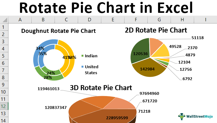
Rotate Pie Chart in Excel | How to Rotate Pie Chart in Excel?

Create a chart from start to finish - support.microsoft.com Data that is arranged in one column or row on a worksheet can be plotted in a pie chart. Pie charts show the size of items in one data series, proportional to the sum of the items. The data points in a pie chart are shown as a percentage of the whole pie. Consider using a pie chart when: You have only one data series.

Create Outstanding Pie Charts in Excel | Pryor Learning

Pie Chart Examples | Types of Pie Charts in Excel with Examples It is similar to Pie of the pie chart, but the only difference is that instead of a sub pie chart, a sub bar chart will be created. With this, we have completed all the 2D charts, and now we will create a 3D Pie chart. 4. 3D PIE Chart. A 3D pie chart is similar to PIE, but it has depth in addition to length and breadth.

Excel: How to not display labels in pie chart that are 0 ...

How to Use Cell Values for Excel Chart Labels - How-To Geek Select the chart, choose the "Chart Elements" option, click the "Data Labels" arrow, and then "More Options.". Uncheck the "Value" box and check the "Value From Cells" box. Select cells C2:C6 to use for the data label range and then click the "OK" button. The values from these cells are now used for the chart data labels.

How to Make a Pie Chart in Excel & Add Rich Data Labels to ...

How to create a pie chart in Excel - beta.hedbergandson.com Step 1: Highlight the data to chart. Step 2: In INSERT-> select the icon of the pie chart -> choose the type of chart to draw, in this example, select the pie chart 2 - D Pie. Step 3: After selecting the chart type, the pie chart is drawn as shown: - In case you want to change the data on a spreadsheet -> the chart updates itself with that change.

Change color of data label placed, using the 'best fit ...

How to add or move data labels in Excel chart? - ExtendOffice In Excel 2013 or 2016. 1. Click the chart to show the Chart Elements button . 2. Then click the Chart Elements, and check Data Labels, then you can click the arrow to choose an option about the data labels in the sub menu. See screenshot: In Excel 2010 or 2007. 1. click on the chart to show the Layout tab in the Chart Tools group. See ...

EXCEL Charts: Column, Bar, Pie and Line

How to add data labels from different column in an Excel chart? Right click the data series in the chart, and select Add Data Labels > Add Data Labels from the context menu to add data labels. 2. Click any data label to select all data labels, and then click the specified data label to select it only in the chart. 3.

How to fix wrapped data labels in a pie chart | Sage Intelligence

How to Add Data Labels to an Excel 2010 Chart - dummies Use the following steps to add data labels to series in a chart: Click anywhere on the chart that you want to modify. On the Chart Tools Layout tab, click the Data Labels button in the Labels group. None: The default choice; it means you don't want to display data labels. Center to position the data labels in the middle of each data point.

Change the format of data labels in a chart

How to Create and Format a Pie Chart in Excel - Lifewire To add data labels to a pie chart: Select the plot area of the pie chart. Right-click the chart. Select Add Data Labels . Select Add Data Labels. In this example, the sales for each cookie is added to the slices of the pie chart. Change Colors

How to Create a Pie Chart in Excel | Smartsheet

Histogram - Examples, Types, and How to Make Histograms Let us create our own histogram. Download the corresponding Excel template file for this example. Step 1: Open the Data Analysis box. This can be found under the Data tab as Data Analysis: Step 2: Select Histogram: Step 3: Enter the relevant input range and bin range. In this example, the ranges should be:

How to Make Pie Chart with Labels both Inside and Outside ...

excel - Positioning data labels in pie chart - Stack Overflow Positioning data labels in pie chart. I'm trying to format some charts I have, using VBA. To get started I recorded a macro of me doing what I wanted, to have an idea of what methods I'd want etc. The recorded macro looks like this - I'm including the whole thing, though the line to pay attention to is Selection.Position = xlLabelPositionCenter.

Appian Community

Office: Display Data Labels in a Pie Chart - Tech-Recipes: A Cookbook ... 2. If you have not inserted a chart yet, go to the Insert tab on the ribbon, and click the Chart option. 3. In the Chart window, choose the Pie chart option from the list on the left. Next, choose the type of pie chart you want on the right side. 4. Once the chart is inserted into the document, you will notice that there are no data labels.

How to Add Data Labels to your Excel Chart in Excel 2013

Creating Pie Chart and Adding/Formatting Data Labels (Excel) Creating Pie Chart and Adding/Formatting Data Labels (Excel) Creating Pie Chart and Adding/Formatting Data Labels (Excel)

How to Create a Pie Chart in Excel - Displayr

How to Create a Pie Chart in Excel: A Quick & Easy Guide - wikiHow You need to prepare your chart data in Excel before creating a chart. To make a pie chart, select your data. Click Insert and click the Pie chart icon. Select 2-D or 3-D Pie Chart. Customize your pie chart's colors by using the Chart Elements tab. Click the chart to customize displayed data. Part 1.