38 excel column chart labels
How to Add Labels to Scatterplot Points in Excel - Statology Next, click anywhere on the chart until a green plus (+) sign appears in the top right corner. Then click Data Labels, then click More Options… In the Format Data Labels window that appears on the right of the screen, uncheck the box next to Y Value and check the box next to Value From Cells. How to Print Labels from Excel - Lifewire To label legends in Excel, select a blank area of the chart, select the Plus ( +) in the upper-right, and check the Legend checkbox. Then, select the cell containing the legend and enter a new name. How do I label a series in Excel? To label a series in Excel, right-click the chart with the data series and choose Select Data.
Excel Waterfall Chart: How to Create One That Doesn't Suck Click inside the data table, go to " Insert " tab and click " Insert Waterfall Chart " and then click on the chart. Voila: OK, technically this is a waterfall chart, but it's not exactly what we hoped for. In the legend we see Excel 2016 has 3 types of columns in a waterfall chart: Increase. Decrease.

Excel column chart labels
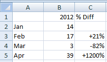
Custom Chart Data Labels In Excel With Formulas Follow the steps below to create the custom data labels. Select the chart label you want to change. In the formula-bar hit = (equals), select the cell reference containing your chart label's data. In this case, the first label is in cell E2. Finally, repeat for all your chart laebls. Chart.ApplyDataLabels method (Excel) | Microsoft Docs Syntax Parameters Example Applies data labels to all the series in a chart. Syntax expression. ApplyDataLabels ( Type, LegendKey, AutoText, HasLeaderLines, ShowSeriesName, ShowCategoryName, ShowValue, ShowPercentage, ShowBubbleSize, Separator) expression A variable that represents a Chart object. Parameters Example How to Show Percentages in Stacked Column Chart in Excel? By default, the data labels are shown in the form of chart data Value (Image 1). But very often user needs to plot charts with actual data and show percentages/custom values on the chart instead of default data. For that we have an option "Value From Cells" in chart "Format Data Label" (Image 2) to select a custom range. Image 1 Image 2
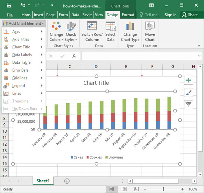
Excel column chart labels. Labeling X-Y Scatter Plots (Microsoft Excel) I think Excel 2013 may have solved this problem. Create the scatter chart from the data columns (cols B and C in this example). Right click a data point on the chart and choose Format Data Labels In the Format Data Labels panel which appears, select Label Options at the top and then the last (column chart) icon (Label Options) just below. How to Add Axis Titles in a Microsoft Excel Chart Select your chart and then head to the Chart Design tab that displays. Click the Add Chart Element drop-down arrow and move your cursor to Axis Titles. In the pop-out menu, select "Primary Horizontal," "Primary Vertical," or both. If you're using Excel on Windows, you can also use the Chart Elements icon on the right of the chart. TickLabels object (Excel Graph) | Microsoft Docs To change the tick-mark label text for the value axis, you must change the values of these properties. Use the TickLabels property to return the TickLabels object. Example The following example sets the number format for the tick-mark labels on the value axis in the chart. VB myChart.Axes (xlValue).TickLabels.NumberFormat = "0.00" See also Two-Level Axis Labels (Microsoft Excel) - ExcelTips (ribbon) Place your row labels into column A, beginning at cell A3. Place your data into the table, beginning at cell B3. With your table completed, you are ready to create the chart. Just select your data table, including all the headings in the first two rows, then create your table.
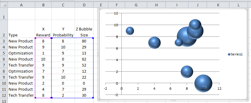
Excel Line Column Chart With 2 Axes - Contextures Excel Tips On the Excel Ribbon, click Insert tab, then click Column Chart In the 2-D Column section, click the first chart type -- 2D Clustered Column chart This creates a chart that is embedded on the active worksheet, with both the series shown as columns. Product names are shown in the axis labels on the horizontal axis 5 New Charts to Visually Display Data in Excel 2019 - dummies Arrange the data sets in columns, with a separate column for each data set. Place text labels describing the data sets above the data. Select the data sets and their column labels. Click Insert → Insert Statistic Chart → Box and Whisker. Format the chart as desired. Box and whisker charts are visually similar to stock price charts, which ... Excel: How to Create a Bubble Chart with Labels - Statology Step 3: Add Labels. To add labels to the bubble chart, click anywhere on the chart and then click the green plus "+" sign in the top right corner. Then click the arrow next to Data Labels and then click More Options in the dropdown menu: In the panel that appears on the right side of the screen, check the box next to Value From Cells within ... Excel Pivot values as column labels - Stack Overflow If you have Excel for Office 365 (or Excel 2021) with the FILTER function, you can use the following: Note that I used a table with structured references for the data source. This has advantages in editing the table in the future. For "pivot" header: =TRANSPOSE(SORT(UNIQUE(Table1[Country]))) For the columns:
Horizontal axis labels on a chart - Microsoft Community If you start with Jan or January, then fill down, Excel should automatically fill in the following names. Click on the chart. Click 'Select Data' on the 'Chart Design' tab of the ribbon. Click Edit under 'Horizontal (Category) Axis Labels'. Point to the range with the months, then OK your way out. --- Kind regards, HansV 8 Types of Excel Charts and Graphs and When to Use Them Pie graphs are some of the best Excel chart types to use when you're starting out with categorized data. With that being said, however, pie charts are best used for one single data set that's broken down into categories. If you want to compare multiple data sets, it's best to stick with bar or column charts. 3. Build a Panel Chart in Excel - Step-by-step Tutorial with Example Step 3: Build a Pivot Table from the data. Steps to build a new Pivot Table: Select the range of cells, in this case, cell C3. Click on the Insert Tab. Click PivotTable. Now in the 'Create PivotTable' dialog box, apply the following settings. We want to manage the original data set and the new Pivot data in the same Worksheet. How to Create a Dynamic Chart Title in Excel Steps to Create Dynamic Chart Title in Excel. Converting a normal chart title into a dynamic one is simple. But before that, you need a cell which you can link with the title. Here are the steps: Select chart title in your chart. Go to the formula bar and type =. Select the cell which you want to link with chart title.
Excel-User.com: Excel Charts - Add totals labels to Stacked Column chart
How to Use Excel Pivot Table Label Filters Right-click on an item in the Row Labels or Column Labels In the pop-up menu, click Filter, then click Hide Selected Items. The item is immediately hidden in the pivot table. Quickly Hide All But a Few Items You can use a similar technique to hide most of the items in the Row Labels or Column Labels.
:max_bytes(150000):strip_icc()/Capture-6f4479134153400a9f234f5a11375bce.JPG)
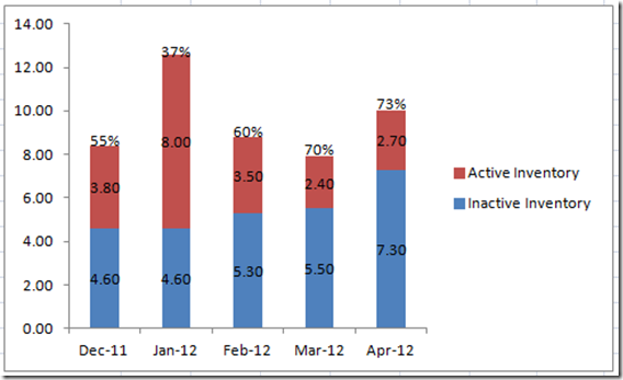
Change Column Colors / Show Percent Labels in Excel Column Chart
How to Create a Run Chart in Excel (2021 Guide) | 2 Free Templates How to Create a Run Chart in Excel Step 1. Calculate the Median Step 2. Build a Line Chart Step 3. Spruce Up Your Run Chart 2 Excel Run Chart Templates 1. Defect Trend Run Chart Template 2. Run Chart with Dynamic Data Labels Run Charts: Overview
3d scatter plot for MS Excel
How do you label data points in Excel? - profitclaims.com Right click the data series in the chart, and select Add Data Labels > Add Data Labels from the context menu to add data labels. 2. Click any data label to select all data labels, and then click the specified data label to select it only in the chart. 3.

Improve your X Y Scatter Chart with custom data labels
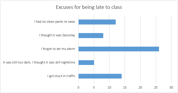
How can I get data labels to show for each column in a bar chart? Turn on 'Overflow text' under Data label' Format tab. Also, you can adjust the position of the Data Label by switching to 'Outside End' or 'Inside Center' so that your Data Label gets displayed properly. If this post helps, then mark it as 'Accept as Solution ' so that it could help others. Regards, Sanket Bhagwat View solution in original post
Dynamically Change Excel Bubble Chart Colors - Excel Dashboard Templates
How to Apply a Filter to a Chart in Microsoft Excel RELATED: How to Create and Customize a Funnel Chart in Microsoft Excel. Select the data for your chart, not the chart itself. Go to the Home tab, click the Sort & Filter drop-down arrow in the ribbon, and choose "Filter." Click the arrow at the top of the column for the chart data you want to filter.
How To Make a Chart In Excel | Deskbright
Add or remove data labels in a chart - Microsoft Support

What's new in Excel 2013 - Excel
Bar Chart in Excel - Types, Insertion, Formatting - Excel Unlocked To add Data Labels to the chart, perform the following steps:- Click on the Chart and go to the + icon at the top right corner of the chart. Mark the Data Labels from there After that, select the Horizontal Axis and press the delete key to delete the horizontal axis scale. This is how the chart looks once finished.
How to Add an Axis Title to an Excel Chart | Techwalla
Format Chart Axis in Excel - Axis Options Right-click on the Vertical Axis of this chart and select the "Format Axis" option from the shortcut menu. This will open up the format axis pane at the right of your excel interface. Thereafter, Axis options and Text options are the two sub panes of the format axis pane. Formatting Chart Axis in Excel - Axis Options : Sub Panes

Excel-User.com: Excel Charts - Add totals labels to Stacked Column chart
Modifying Axis Scale Labels (Microsoft Excel) Follow these steps: Create your chart as you normally would. Double-click the axis you want to scale. You should see the Format Axis dialog box. (If double-clicking doesn't work, right-click the axis and choose Format Axis from the resulting Context menu.) Make sure the Number tab is displayed. (See Figure 1.)
How-to Add Custom Labels that Dynamically Change in Excel Charts - Excel Dashboard Templates
How to Create a Pie Chart from a Single Column [FREE Template ... Step 2. Create a Pie Chart from the Pivot Table. With everything we need in place, it's time to create a pie chart Excel using the pivot table you just built. Select any cell in your pivot table (C1:D12). Navigate to the Insert tab. Hit the "Insert Pie or Doughnut Chart" button. Under "2-D Pie," click "Pie."

34 Excel Chart Label Axis - Labels 2021
How to Show Percentages in Stacked Column Chart in Excel? By default, the data labels are shown in the form of chart data Value (Image 1). But very often user needs to plot charts with actual data and show percentages/custom values on the chart instead of default data. For that we have an option "Value From Cells" in chart "Format Data Label" (Image 2) to select a custom range. Image 1 Image 2

34 Label Columns In Excel - Labels For You
Chart.ApplyDataLabels method (Excel) | Microsoft Docs Syntax Parameters Example Applies data labels to all the series in a chart. Syntax expression. ApplyDataLabels ( Type, LegendKey, AutoText, HasLeaderLines, ShowSeriesName, ShowCategoryName, ShowValue, ShowPercentage, ShowBubbleSize, Separator) expression A variable that represents a Chart object. Parameters Example
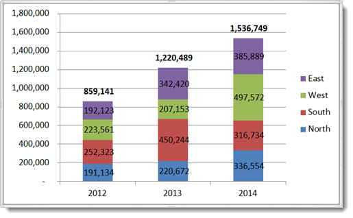
How-to Put Percentage Labels on Top of a Stacked Column Chart - Excel Dashboard Templates
Custom Chart Data Labels In Excel With Formulas Follow the steps below to create the custom data labels. Select the chart label you want to change. In the formula-bar hit = (equals), select the cell reference containing your chart label's data. In this case, the first label is in cell E2. Finally, repeat for all your chart laebls.

35 How To Label A Column In Excel - Labels Database 2020
Bar Chart in Excel - Easy Excel Tutorial
How to Show Percentages in Stacked Bar and Column Charts in Excel
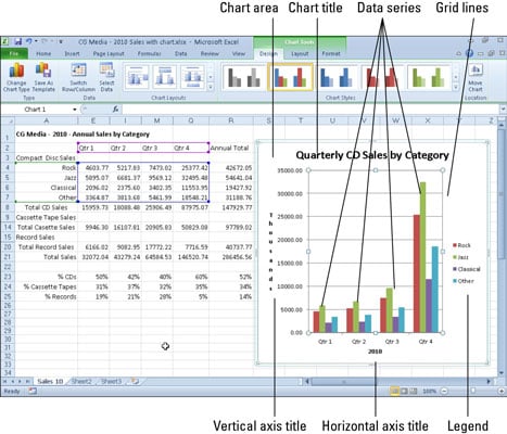
Getting to Know the Parts of an Excel 2010 Chart - dummies
Post a Comment for "38 excel column chart labels"